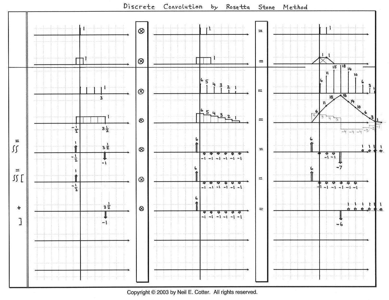
| Tool: | We can calculate discrete convolutions as continuous-time convolutions if we replace each sample value with a rectangle function centered over the sample. As shown in the diagram below in the first two lines, the convolution of the rectangle functions produces triangle functions in the final answer. The peak height of each triangle is the value of the discrete sample in the final answer. |
| The advantage of using a continuous-time convolution is that flat sections of a discrete waveform become side-by-side rectangle functions that equal one wider rectangle function. Then we can employ the technique of DIFFERENTIATED CONVOLUTION INTEGRALS to find our final answer. | |
| Ex: | In lines 3-7 below, we show an example where four samples become four rectangle functions that become one rectangle function in line 4. We then differentiate both of the waveforms being convolved, resulting in a convolution of sets of impulses in line 5. In lines 6 and 7, we compute the convolution from line 5 by employing the replicating property of convolution with impulse (i.e., delta) functions. We sum the results of lines 6 and 7 to get the answer for line 5. Then we integrate twice to get the answer on line 4. We sample the result in line 4 to get the same answer we would get from a discrete convolution. |
|
|