Tool: The FFT (Fast Fourier Transform) exploits the repetition of values of complex exponentials to reduce the number of calculations required for a DFT (Discrete Fourier Transform).
The DFT equation is
![]()
where
![]() .
.
The fundamental idea underlying the FFT is that, since W1/N is the Nth root of unity, W1/N raised to the Nth power is equal to unity:
![]() .
.
When kn exceeds N, we start repeating values of the complex exponential. Thus, we have only N distinct values of the complex exponential, repeated numerous times. We save calculations by finding terms that will be multiplied by the same value of complex exponential and summing them first.
The rote procedure for developing an FFT is to write nk as a multiple of N plus a remainder. (A subtlety is that the remainder may actually be greater than N, but our algorithm remains valid.) Given a sampled waveform, x(n), of duration N = LM points, we write indices in time and frequency as though the one-dimensional arrays for x(n) and DFT X(k) are stored as two-dimensional arrays:
![]()
Note that n is stored as L columns (indexed by l) and M rows (indexed by m), whereas k is stored as M columns (indexed by q) and L rows (indexed by p). This causes a term of form pMmL = pmN to appear in the product nk.
We proceed by using our new definitions for n and k in the DFT:
![]() .
.
(Note that the summations may be in either order. The above order corresponds to a decimation-in-time algorithm, whereas the other order corresponds to a decimation-in-frequency algorithm.) Expanding the exponent of W yields
![]()
Now we rewrite the DFT as nested DFT calculations with some extra "twiddle factors" thrown in:
![]()
To reveal the DFT's, we use a notation that reveals which variable is summed over time, and which variable is summed over frequency.
![]()
Inner
loop: ![]() (DFT
result has L points)
(DFT
result has L points)
![]() (multiply
by twiddle factors)
(multiply
by twiddle factors)
Outer
loop: ![]() (DFT
result has M points)
(DFT
result has M points)
![]()
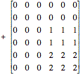
ex: Consider the case of N = 6. We use L = 2 and M = 3. We use matrix notation to reveal the redundancy of the calculations. The DFT may be written as follows where we write all exponents modulo N:
where
![]() .
.
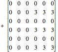
The column index of the matrix corresponds to n = mL + l, and the row index corresponds to k = pM + q. The summations over l and m have the effect of shuffling the rows and columns so that columns with the same value of l are together and rows with the same value of q are together. In other words, build the shuffled matrix from the original by taking every Lth column and every Mth row.
For the shuffling of rows, we have
 .
.
Adding the shuffling of columns, we have
 .
.
Here, we observe redundancy. In the first three columns, every other row is duplicated. In the last three columns, every other row is just w3 times the row above.
If we consider the exponents in the matrix, we may write them as the sum of three matrices whose entries are pMl (mod N), ql (mod N), and qmL (mod N). Note that these terms were the exponents of W early in the derivation of the FFT.
 (matrix
qmL (modN))
(matrix
qmL (modN))
 (matrix
ql (modN))
(matrix
ql (modN))
 (matrix
pMl (modN))
(matrix
pMl (modN))
For the first matrix, we have redundancy that allows us to write the first step of processing (i.e., the first DFT's) as follows:
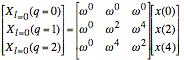 .
.
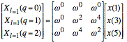 .
.
The second matrix contains the twiddle factors:
![]()
![]()
![]()
The third matrix contains the multipliers for the final step—the computation of the second set of DFT's:
![]()
![]()
![]()
Note: The number of multiplies we use is LM2 + N + ML2 = N(M + L + 1). This compares with N2 for the direct calculation of the DFT. In the above example we break even, but for N = 16 we would have 144 multiplies with the FFT compared to 256 without. As N grows, the savings increase.
Note: If N is highly composite, we can apply the FFT to the smaller DFT's in a recursive fashion. In particular, if N is a power of two we can successively divide N by two until all the DFT's are of size two. It follows that W1/N = W1/2 = –1 for all the DFT's. Thus, we have no multiplies at all (just sign changes) for the DFT's. We still have twiddle factors that are roots of unity, but the total number of multiplies is dramatically smaller than it would be for a direct calculation of the DFT.