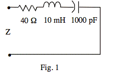
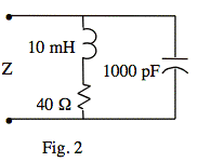
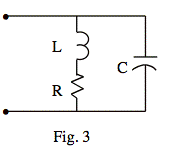
Ex:           Make calculations of |Z| for enough values of ω that you can plot a good graph of |Z| versus ω for each of the circuits shown in Figs. 1 and 2. Then vary the values of the components, and make enough further calculations that you can get a qualitative feel for how the size and shape of the curve depends on the parameters, without making numerical calculations. For example, if |Z| versus ω is given for the circuit shown in Fig. 3, explain how the curve would change if R were doubled, with nothing else changed. Explain how the curve would change if L were doubled, with nothing else changed.

              

Ans:     Fig. 1)   plot of |z| will be bowl-shaped with a minimum value of R at ωo.

Fig. 2)   |z| = R = 40 Ω at ω = 0.

|z| increases to a resonant peak of (approximate) height kR = 6.25 k ⋅ 40 Ω = 250 kΩ. The resonant frequency is 1/√(LC) = 1 M/√10 rad/s.

|z| then decreases toward 0 as ω → ∞.

              Fig. 3)   Double R: |z| starts at twice the height but the resonant peak height is only half as high. The frequency of the resonant peak is unaffected. Double L, then the curve for |z| still starts at height R but the resonant peak height is about twice as high. The frequency of the resonant peak is lowered by a factor of √2.

Sol'n:  Fig. 1)   z = R + jωL + -j/(ωC) = R + j[ωL - 1/(ωC)]

|z|2 = R2 + [ωL - 1/(ωC)]2

We may visualize |z| as the length of the hypotenuse of a right triangle in the complex plane with sides of length R and [ωL - 1/(ωC)].

At the resonant frequency of the L and C, ωo2 = 1/(LC), the L and C act like a wire: ωL - 1/(ωC) = 0. Thus, z = R at ωo.

For z above or below ωo, the magnitude of [ωL - 1/(ωC)] increases. Thus, our plot of |z| will be bowl-shaped with a minimum value of R at ωo.

              Fig. 2)   z = (R + jωL) || 1/(jωC)

Consider the qualitative behavior at key frequencies: (Note that the lower magnitude impedance dominates in a parallel configuration.)

At ω = 0, R + jωL = R and 1/(jωC) = ∞.

Thus, z = R.

At ω = R/L, R + jωL = R(1+j) and 1/(jωC) = -jR[(L/R)/(RC)].

Thus, z = R[(1 + j) || −j(L/R)/(RC)], and z will behave more like the smaller of the parallel terms. If L/R = RC, however, we will have z = R[(1 + j) || −j] = R(1 − j). For the component values given, L/R = 1/4 ms, RC = 40 ns, and (L/R)/(RC) = 6.25 k. It follows that z ≈ R(1+j) at ω = R/L for this circuit.

As ω → ∞, R + jωL → R + j∞ and 1/(jωC) → 0.

Thus, z → 0.

Now we examine the behavior versus frequency more carefully. Our calculations are driven by the thought that the resonance of the L and C may cause the L and C to become almost an open circuit. The R, however, will affect the resonance.

To simplify the algebra, we use normalized (and unitless) frequency ωn = ω/(R/L). We have z = R[(1 + jωn) || −j(L/R)/(RCωn)].

Define k ≡ (L/R)/(RC). Then we have z = R[(1 + jωn) || −jk/ωn] or z = R[(−jk/ωn + k)/(1 + j[ωn −k/ωn])].

Define ωno ≡ √k. At ωn = ωno, we have ω = ωo ≡ 1/√(LC), ωno = k/ωno, and z = R[−jωno + k] = R[−j√k + k].

If k << 1, then z ≈ Rk << R and the L and C do not act like an open circuit at resonance. Instead, the circuit acts like the C is nearly shorted.

If k >> 1, then z ≈ Rk >> R and the L and C almost act like an open circuit at resonance. This case applies to Fig. 2.

Now we have enough information to describe the shape of |z| versus ω as ω goes from 0 to ∞:

|z| = R = 40 Ω at ω = 0.

|z| increases to a resonant peak of (approximate) height kR = 6.25 k ⋅ 40 Ω = 250 kΩ. The resonant frequency is 1/√(LC) = 1 M/√10 rad/s.

|z| then decreases toward 0 as ω → ∞.

              Fig. 3)   Based on calculations for Fig. 2, if we double R then the curve for |z| starts at twice the height but the resonant peak height of Rk is only half as high (since Rk behaves like 1/R). The frequency of the resonant peak is unaffected.

If we double L, then the curve for |z| still starts at height R but the resonant peak height of Rk is about twice as high (since k is proportional to L). The frequency of the resonant peak is lowered by a factor of √2.

Note: These results only apply to the case k >> 1. If R becomes too large, then our approximations break down (and the resonant peak may disappear entirely).