Ex:           Consider the steady-state torque equation for an induction motor, [1], with the parameters listed below:

where         τe  ≡    torque (Nm)

                 np  ≡    number of pole pairs

                  M  ≡    mutual inductance of rotor and stator coils (H)

                RR  ≡    rotor resistance (Ω)

                  IS  ≡    magnitude of stator current (A)

                   S  ≡    slip (rad/s)

                TR  ≡    rotor time constant = LR/RR (s)

                LR  ≡    rotor inductance (H)

Use Matlab to make a plot of slip frequency, S, versus steady-state electrical frequency, ωe. Superimpose a plot of ω versus ωe. Assume the steady-state torque equals friction Bw. (Rewrite ω as ωe − S when solving for S. After you find S, use this equation again to calculate ω.) Use values of ωe in the range [1, 30] rad/s.

Note:      The equation to be solved is a cubic in S. Use the smallest real root as the value of S. The Matlab function roots([1,a,b,c]) finds the roots of the following cubic polynomial:

Motor parameters:

                                    

                                  

Ref:   [1] Marc Bodson, "Control of Electric Motors," 2004, University of Utah ECE Dept., eqn 4.62 p. 130.

 

Sol'n:      Define a convenient constant to simplify notation

Setting τe = Bw and substituting for ω in terms of S, we have

Rearranging gives

Simplifying, we have a cubic equation for S:

We use Matlab to calculate S versus ωe and ω versus ωe, (see code below).

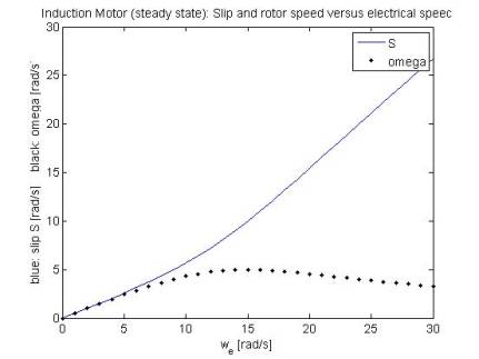
We observe that there is a peak motor speed for ωe ≈ 15 rad/s.

% ECE5570F05prob3soln.m

%

% Matlab code for plotting slip frequency S versus electrical freq w_e.

% For induction motor. Uses eqn 4.62 from "Control of Electric Motors"

% by Marc Bodson.

 

% Set values of motor parameters.

L_R = 2/100; % (H) = inductance of rotor

R_R = 2/10; % (ohms) = resistance of rotor

M = 1/100; % (H) = mutual inductance of stator and rotor

I_s = 200; % (A) = current in stator

J_motor = 5/100; % (kgm^2) = moment of inertia of motor (not used)

np = 1; % (-) = number of pole pairs

 

% Calculate rotor time constant.

T = L_R / R_R;

 

% Use figure 1 for all plots

figure(1)

 

% Create empty w_e_vec array so Matlab accepts later statements.

w_e_vec = [];

 

% Create empty Svec array so Matlab accepts later statements.

Svec = [];

 

% Plot S for values of w_e in range [1,5] rad/s.

for w_e = 0:1:30

 

% Build w_e vec.

w_e_vec = [w_e_vec, w_e];

 

% Set coeffs of polynomial to be solved. Polynomial eqn is:

% S^3 - w_e * S^2 + 2/T^2 * S - w_e/T^2 = 0

poly_coeffs = [1, -w_e, 2/T^2, -w_e/T^2];

 

% Find roots of polynomial.

S_vals = roots(poly_coeffs);

 

% Find real roots.

real_S_vals = S_vals(find(abs(imag(S_vals)) < eps));

 

% Use smallest real root.

S_min = min(real_S_vals);

 

% Add answer to array of S values vs w_e.

Svec = [Svec, S_min];

 

end

 

% Calculate motor speed, omega.

omega = w_e_vec - Svec;

 

% plot results

plot(w_e_vec, Svec, 'b-', w_e_vec, omega, 'k.')

xlabel('w_e [rad/s]')

ylabel('blue: slip S [rad/s] black: omega [rad/s]')