Ex:           Which of the following joint density functions have (correlation) ρXY = 0?

(Remember that ρXY = 0 is possible with symmetry even if X and Y are not independent.)

a)     

b)     

c)      Estimate by eye the value of x for which F(x) = 0.25.

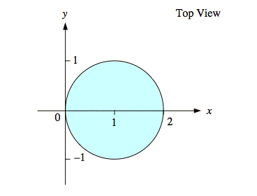
Sol'n: a)  The region, x2 + y2 ≤ 1, on which f(x, y) ≠ 0 is called the support of f(x, y). It is a circle of radius one, centered at x = 1 and y = 0, as shown below.

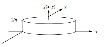
Since f(x, y) = 1/π is constant on its support, f(x, y) is a cylinder as shown below.

By symmetry, we can say that the mean values for x and y are μx = 1 and μy = 0. Since correlation is measured relative to mean values we have the following conceptual tool that allows us to simplify the calculation of ρxy:

Tool:      Variance and covariance terms are always expressed in terms of distances from means:

,                                      

Thus, we get the same values for a probability density function (pdf) such as fX(x) or f(x, y) shifted so that the mean values are at the origin. In other words, slide f(x, y) around on the xy-plane so that μX = 0 and μY = 0. For this shifted f(x, y), the calculation of variances is simplified:

,                

Applying this tool to the present problem yields a new pdf that is a cylinder centered on the origin:

Since correlation is defined in terms of variances and covariance, the correlation of this new f(x, y) will be the same as for the original f(x, y):

The covariance, , appears in the numerator of the definition of correlation, and we examine it first in case we can show it is zero. If we can do so, then it follows that the correlation is zero and we are done.

As noted above, for our new f(x, y). Calculation of E(x, y) involves a double integral:

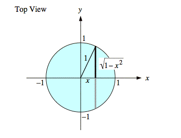
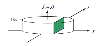
To determine the correct substitutions for the limits of integration, we consider the support of a cross-sections of f(x, y) in the y direction for one value of x, as shown below.

The illustration, below, shows the cross section itself at this same value of x.

From the diagrams we have the following integral:

Rather than calculating the inner integral, we observe that it is the integral of an odd function, (i.e., g(y) = −g(−y)), with equal but opposite limits of integration. In other words, the value of the integrand at y is equal to minus one times the value of the integrand at −y. Thus, these two points cancel each other out in the integral. This happens at every value of y, and it follows that the integral is zero.

We can verify this result by hand or by using the following Matlab® commands to compute the integral:

syms x y

int(x*y/pi,y,-sqrt(1-x^2),sqrt(1-x^2))

Since the covariance is zero, it follows that the correlation is zero:

             b) The correlation for this joint probability density function is zero since X and Y are independent.

To show independence of X and Y, we write f(x, y) as the product of fX(x) and fY(y).

Note:      We are able to separate the conditions on x and y for this f(x, y). This is possible because the conditions on x (i.e., 1 ≤ x ≤ 2) do not include y and vice versa. If the conditions for x depend on the value of y or vice versa, then X and Y are almost certainly dependent.

             c)  We suspect the correlation for this joint probability density function is nonzero since X and Y are dependent. The dependence of X and Y is revealed by taking cross-sections and seeing that they have different shapes after being scaled vertically to make their area equal one. That is, the conditional probabilities change with the value of the variable being conditioned on.

Any hoped for symmetry is elusive, as the mean values in the x and y directions are not immediately apparent, and turn out to be awkward values:

Note that the quantity in the parentheses in the last integral is fX(x), which we will use below.

By symmetry we have μY = μX = 7/12. These values are awkward because they are not in the center of the figure. Thus, it seems unlikely that we will be able to pair up all points in such a way that they cancel out in calculation of correlation.

We proceed with the calculation of variances and covariance needed for the calculation of correlation.

Subtract the mean squared to find the variance:

By symmetry the variance is the same for Y.

Now compute the covariance. The first step is to find E(XY).

or

Now subtract the product of the means.

Now we plug values into the formula for correlation:

The correlation is nonzero but very small.