|
|
By: Neil E. Cotter |
Probability |
|
|
|
Designing pdf's |
|
|
|
Example 2 |
|
|
|
|
|
|
|
|
Ex: (This problem is motivated by problem of using the rand( ) function in Matlab® to create arbitrary probability density functions.) Given three independent random variables, V, W, and Z, that are uniformly distributed on [0, 1], describe a step-by-step calculation that yields random variables X and Y with the following joint density function (whose footprint is shaped like a diamond centered on the origin):

Hint: First generate X from the density function fX(x) using some simple algebra involving V and W. Then generate Y from the conditional probability density function f(y | X). Use Z and some simple algebra to create Y.
Sol'n: The plot below shows the support (or footprint) of f(x, y).
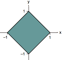
Fig. 1. Support (or footprint) of f(x, y).
In a 3-dimensional view, the diamond shape of f(x, y) has a constant height of 1/2.
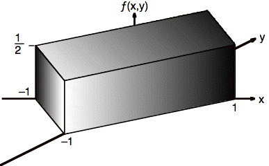
Fig. 2. 3-dimensional plot of f(x, y).
The rationale for the hint is that we can write the joint probability, f(x, y), as the product of a density function for x alone and a conditional probability for y given x:
![]()
This means that we can first pick X distributed as fX(x) and then pick Y distributed as f(y | X).
To find fX(x), we use the standard formula for integration in the y direction:
![]()
Fig. 3, below, shows the limits of the integral for a particular value of x = xo as the endpoints of a cross-section in the y direction. The value of f(x, y) over this segment is one‑half.
![]()
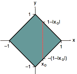
Fig. 3. Top view of cross-section used to calculate fX(xo) and f(y | X = xo).
This above formula, written using absolute value, actually holds for any positive or negative value of xo, and we have the following formula for probability density of X:
![]()
Fig. 4 shows that fX(x) is triangular.
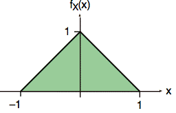
Fig. 4. Plot of fX(x).
There are two straightforward ways to generate a random variable, X, with this probability density function. The first is to add two uniformly distributed random variables together (and subtract one to give a mean of zero):
![]()
The probability density function for X is computed as a convolution integral. We start with the probability density of V and find the probability density that W = X − (V − 1). We integrate this product over possible values of V.
![]()
We observe that fW(w) = 1 when 0 < w < 1.
![]()
Rearranging the inequality to express it in terms of v yields the following expression:
![]()
Substituting fV(v) = 1 and translating the expression for fW(w) into modifications of the limits of integration yields the following expression for the density function shown in Fig. 4:
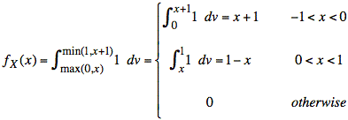
From the above discussion, the step-by-step procedure for calculating X is to use the following simple formula:
![]()
Another way to obtain a random variable with the density function shown in Fig. 4 is to transform a single uniform random variable such as V by matching the cumulative distribution functions of X and V.
The cumulative distribution function for V is easily computed:

The cumulative distribution function for X is quadratic since fX(x) is linear.
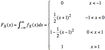
Given a value for V, we find a value of X such that FX(x) = FV(V). This translates in the following equation:

or

Now that we have X, we use the conditional probability density function, f(y | X) for Y. We find f(y | X) by first taking a cross section of f(x, y) at x = X, as shown in Fig. 5.
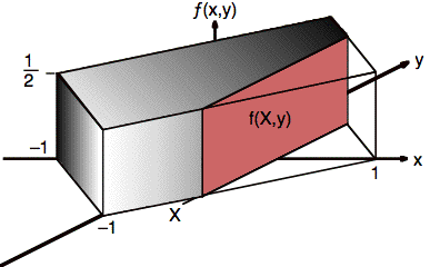
Fig. 5. Cross-section used to calculate fX(X) and f(y | X).
We scale the cross section vertically so it will have a total area equal to one. Fig. 6 shows the result.
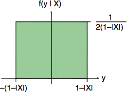
Fig. 6. Conditional probability f(y | X).
We obtain this distribution by shifting and scaling a (0,1) uniform distribution such as Z.
![]()