Ex:           Using Matlab® or pencil and paper, make an accurate plot of a standard gaussian distribution and answer the following questions:

a)      What is the value of f(x) at x = 0?

b)      At what value of x does f(x) = 0.5?

c)      Estimate by eye the value of x for which F(x) = 0.25.

d)      Use a table of area under the normal (i.e., gaussian) curve to find the value of x for which F(x) = 0.25.

e)      Use a table of area under the normal (i.e., gaussian) curve to find P(1 ≤ x ≤ 2).

Sol'n: a)  The standard gaussian has μ = 0 and σ2 = 1:

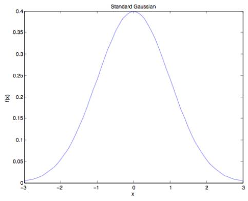
The value of f(x) at x = 0 is the constant term since e0 = 1:

≈ 0.3989 = 0.4

             b) From the plot, we observe that f(x) never reaches a value of 0.5.

             c)  F(x) is the cumulative distribution function, which is equal to the area under the probability function to the left of x. Thus, we are looking for the value of x where the area to the left of x is 1/4 of the total area of the probability density function, (since the total area under the probability density function is equal to one).

The author's estimate is x ≈ −3/4.

             d) Since we have a standard gaussian, we may use a table for the area under a standard gaussian directly. Note that such tables give values of F(x). We use the table in reverse, however. We look for the value of F(x) = 0.25 in the table and then look at the value of x that corresponds to that F(x). The value we obtain is −0.675 to three significant figures.

             e)  P(1 ≤ x ≤ 2) = P(x ≤ 2) − P(1 ≤ x) = F(x = 2) − F(x = 1). Using a table for the area under a standard gaussian, we have

F(x = 2) = 0.9772 and F(x = 2) = 0.8413.

Thus,

P(1 ≤ x ≤ 2) = 0.9772 − 0.8413 = 0.1359.