CONCEPTUAL TOOLS
|
By: Neil E. Cotter
|
Probability
|
|
|
|
Prob density func, f(x) |
|
|
|
Chi-squared
distribution
|
|
|
|
χ2 derivation
|
|
|
|
|
Deriv: The
following is a simplified derivation showing that the probability density
function (pdf) for the normalized sample variance, ![]() , is
the χ2-distribution with n = n
– 1 degrees of freedom where n is the number of independent, normally
distributed samples, s2 is
the variance of each sample, and sample variance s2 is defined in the standard way:
, is
the χ2-distribution with n = n
– 1 degrees of freedom where n is the number of independent, normally
distributed samples, s2 is
the variance of each sample, and sample variance s2 is defined in the standard way:
![]() (1)
(1)
where the Xi are the samples, and ![]() is the sample mean
defined in the standard way:
is the sample mean
defined in the standard way:
![]() . (2)
. (2)
To improve
clarity and focus attention on key ideas in the derivation, we assume the
samples are drawn from a standard normal distribution with mean μ = 0 and variance σ2 = 1:
![]() . (3)
. (3)
Based on rules for linear combinations of random variables, the sample mean is normally distributed with variance s2/n = 1/n since we are assuming s2 = 1.
![]() (4)
(4)
The pdf for
all the samples is an n-dimensional
normal distribution [1].
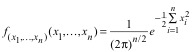 (5)
(5)
With some
manipulation of summations [2], we may show that the summation of the squared xi's may be
written in terms of the sample variance and sample mean:
![]() . (6)
. (6)
or
![]() . (7)
. (7)
Using (6), we
rewrite the n-dimensional normal
distribution:
![]() . (8)
. (8)
We find the pdf
of x = (n – 1)s2 by taking the derivative of the cumulative
distribution function.
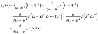 (9)
(9)
Given (8) and
(9), our goal will be to express P(S ≤ s)
in terms of s, but our starting point
is to find the cumulative probability by integrating the pdf of (x1, ..., xn) over all the (x1, ..., xn) that would give a sample variance
that is less than or equal to s2.
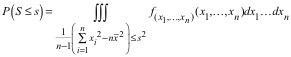 (10)
(10)
or
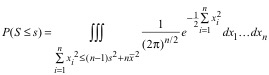 (11)
(11)
We observe
that the pdf ![]() is
spherically symmetric, which suggests that we might be able to use spherical
coordinates for our integral. However,
the spherical symmetry of
is
spherically symmetric, which suggests that we might be able to use spherical
coordinates for our integral. However,
the spherical symmetry of ![]() is with respect
to the origin, whereas we want to integrate over the (x1, ..., xn)
that are within a certain squared distance from
is with respect
to the origin, whereas we want to integrate over the (x1, ..., xn)
that are within a certain squared distance from ![]() . That is, (n – 1)s2 may be thought of as a measure of the squared
distance from (x1,
..., xn) to (
. That is, (n – 1)s2 may be thought of as a measure of the squared
distance from (x1,
..., xn) to (![]() , ...,
, ..., ![]() ):
):
![]() . (12)
. (12)
It follows
that the (x1,
..., xn) are points in an n‑dimensional sphere centered at ![]() at a squared distance
of at most (n – 1)s2 or a radius of
at a squared distance
of at most (n – 1)s2 or a radius of ![]() .
.
For a given ![]() , however, these (x1,
..., xn) must also lie on the hyper-plane of
points such that
, however, these (x1,
..., xn) must also lie on the hyper-plane of
points such that ![]() since the
average of the xi is
since the
average of the xi is ![]() . This plane is
perpendicular to
. This plane is
perpendicular to ![]() or a vector in the
(1,1,1) direction. Thus, for a given
or a vector in the
(1,1,1) direction. Thus, for a given ![]() , we are integrating over the intersection of an n-dimensional sphere of radius
, we are integrating over the intersection of an n-dimensional sphere of radius ![]() and a
hyper-plane in n dimensions that is
perpendicular to the (1,1,1) direction.
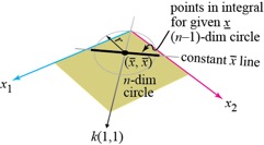
The resulting intersection is an (n–1)-dimensional
sphere. As shown in Fig. 1(a), for the case
of n = 2, (2-dimensional space for X1, X2), the (n–1)-sphere is a 1-dimensional line of
points on the constant
and a
hyper-plane in n dimensions that is
perpendicular to the (1,1,1) direction.
The resulting intersection is an (n–1)-dimensional
sphere. As shown in Fig. 1(a), for the case
of n = 2, (2-dimensional space for X1, X2), the (n–1)-sphere is a 1-dimensional line of
points on the constant ![]() line, and as
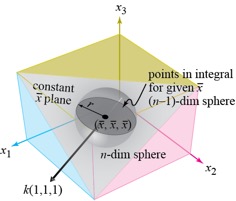
shown in Fig. 1(b), for the case of n
= 3, (3‑dimensional space for X1,
X2, X3), the (n–1)-sphere is a
line, and as
shown in Fig. 1(b), for the case of n
= 3, (3‑dimensional space for X1,
X2, X3), the (n–1)-sphere is a
2-dimensional circle of points on the constant ![]() plane.
plane.
We may use ![]() and r as orthogonal variables of
integration. As we vary
and r as orthogonal variables of
integration. As we vary ![]() ,
the line of constant
,
the line of constant ![]() moves a distance
moves a distance ![]() in the (1,1) direction, and sphere
of integrated points moves with it. This
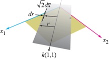
gives an extruded (n–1)-dimensional sphere as the region of integration. As shown in Fig. 2(a) for the case of n = 2, the region of integration is an
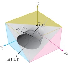
infinite band in the (1,1) direction, and as shown in Fig. 2(b) for the case of
n = 3, the region of integration is
an infinite cylinder in the (1,1,1) direction.
in the (1,1) direction, and sphere
of integrated points moves with it. This
gives an extruded (n–1)-dimensional sphere as the region of integration. As shown in Fig. 2(a) for the case of n = 2, the region of integration is an
infinite band in the (1,1) direction, and as shown in Fig. 2(b) for the case of
n = 3, the region of integration is
an infinite cylinder in the (1,1,1) direction.
(a) (b)
Fig. 1. Points to integrate in the r direction for calculation of P(S
≤ s) at a given value of ![]() :
:
(a) 2-dimensional case, (b) 3-dimensional case.
(a) (b)
Fig. 2. Region of integration for calculation of P(S
≤ s) in coordinates of ![]() and r:
and r:
(a) 2‑dimensional case is infinite band parallel to (1,1) direction,
(b) 3-dimensional case is infinite cylinder parallel to (1,1,1) direction.
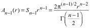
For n ≥ 2 dimensions, the above picture
generalizes to the following change of variables:
![]() . (13)
. (13)
where ![]() varies from –∞ to ∞
and An–1(r) is the surface area of an (n–1)-dimensional sphere of radius
varies from –∞ to ∞
and An–1(r) is the surface area of an (n–1)-dimensional sphere of radius ![]() .
.
From [3] we
have the following formulas for sphere volumes and surface areas:
![]() is
the volume of an n-dimensional sphere
of radius r (14)
is
the volume of an n-dimensional sphere
of radius r (14)
 is
the surface area of an n-dimensional
sphere of radius = 1. (15)
is
the surface area of an n-dimensional
sphere of radius = 1. (15)
It follows
that the surface area of an n-dimensional
unit sphere is:
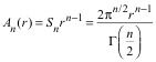 . (16)
The gamma
function has the following properties [4]:
![]() for n
> 0 a positive integer
for n
> 0 a positive integer
![]() for all complex z except integers ≤ 0
for all complex z except integers ≤ 0
![]()
Using (16),
we have:
 . (17)
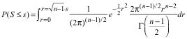
We now have
the following integral for P(S ≤ s):
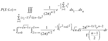 . (18)
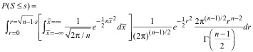
We separate
variables, and perform the inner integration first (after ensuring that the
inner integration is of a normal density function, thus yielding a value of
unity).
 (19)
(19)
The value
inside the square brackets is our integral (of a normal density function) that
has a value of unity. Thus, we have
 . (20)
We now use ν = n – 1 as the "degrees of freedom" to simplify the
expression and reflect the idea that the pdf is analogous to one for n – 1 variables.
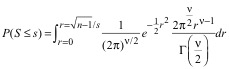 (21)
(21)
Fortunately,
we will take the derivative of the cumulative distribution, so computing the
integral is unnecessary. However, we do
have to deal with a change of variables for the derivative.
As a
preliminary to using the chain rule, we have the following calculations:
![]() (22)
(22)
so
![]() (23)
(23)
and
![]() . (24)
. (24)
Using the
chain rule, we have the following result:
 . (25)
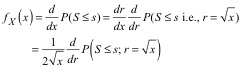
The final
derivative is the derivative of an integral, so the final derivative is just
the integrand from (21):
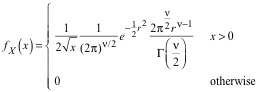 (26)
(26)
or, since r2 = x
and several constants cancel out,
 . (27)
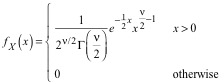
In conclusion, the distribution of x = (n – 1)s2 when s2 = 1 is a chi-squared distribution. Without proof, we state the following result when s2 ≠ 1:
The
probability density function of ![]() is a
chi-squared distribution with n = n – 1 degrees of freedom [2]:
is a
chi-squared distribution with n = n – 1 degrees of freedom [2]:
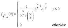 (28)
(28)
Ref: [1] "The Multivariate Normal
Distribution." http://www.math.uah.edu/stat/special/MultiNormal.html
[2] Ronald
E. Walpole, Raymond H. Myers, Sharon L. Myers, and Keying Ye, Probability and Statistics for Engineers and
Scientists, 8th Ed., Upper Saddle River, NJ: Prentice Hall, 2007.
[3] Weisstein, Eric W. "Hypersphere."
From MathWorld--A
Wolfram Web Resource. http://mathworld.wolfram.com/Hypersphere.html
[4] Weisstein, Eric W. "Gamma Function." From MathWorld--A Wolfram Web Resource. http://mathworld.wolfram.com/GammaFunction.html