Tutorial:   STATE VARIABLES and MATLAB^®

Time-domain analysis of circuits with more than one L and C is difficult because it requires solution of characteristic equations higher than second degree. This supplement illustrates the use of Matlab^® functions, ode23 and ode45, for solving a system of coupled first-order differential equations of the form

                dx/dt = f(x,t)

where x is a vector called the state vector, and t is the independent variable, which in our case will be time. As indicated in Mastering Matlab^® 7, Chapter 25, a differential equation can always be expressed as a system of coupled first-order differential equations. The Matlab^® functions are powerful because they can be used to solve nonlinear as well as linear differential equations.

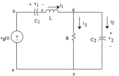
Consider the third-order circuit in Fig. 1 as an example for illustrating the use of the state vector (state variables) and ode45. Let's use Matlab^® to plot v2 as a function of time. Using Kirchhoff's laws in the time domain, we could write the third-order differential equation for v2 and then convert it to three coupled first-order equations following the procedure outlined in the Matlab^® book. It is much easier, however, to obtain the system of coupled first-order equations directly in terms of what are called the state variables. For circuits, the state variables are the currents through inductances and the voltages across capacitances. Using Kirchhoff's laws in the time domain, it is easy to write first-order differential equations in terms of these variables because i = C dv/dt for a capacitance, and v = L di/dt for an inductance, both of which involve first derivatives.

   

Fig. 1. Third-order circuit. vg(t) is a step function that switches from −v0 to v0 at t = 0.

The state variables for the circuit in Fig. 1 are v1, v2, and i1. The first equation is easily obtained from the relationship between the voltage and current for C1:

(1)           dv1/dt = i1/C

The second equation is obtained by writing Kirchhoff's voltage equation around the closed path abcdea :

                -vg + v1 + L di1/dt + v2 =0

from which we get

(2)           di1/dt = − v1/L − v2/L + vg/L

The third equation is obtained by using Kirchhoff's current law,

                i1 = i2 + i3

and i3 = v2/R, i2 = C2 dv2/dt to get

(3)           dv2/dt = i1/C2 - v2/RC2

Now defining the state vector (note that x is a column vector) as

(4)           x = [ v1 i1 v2]'

we get the three coupled first-order differential equations from (1), (2), (3), and (4):

(5)           dx1/dt = x2/C1

(6)           dx2/dt = − x1/L − x3/L + vg/L

(7)           dx3/dt = x2/C2 − x3/RC2

Before writing the Matlab^® program, we need the initial conditions on the vector x. The initial conditions for x are much easier to obtain than for the third-order differential equation for v2. Because the current cannot change instantaneously through an inductance, and because the voltage across a capacitance cannot change instantaneously,

                v1(0+) = v1(0-) = −v0

                i1(0+) = i1(0-) = 0

                v2(0+) = v2(0-) = 0

The initial value of x is thus

(8)           x0 = [−v0 0 0]'

The ode45 function requires a function that calculates xdot (which stands for dx/dt) as a function of t and x (see Matlab^® book). Here is a function that calculates xdot as described by (5)-(7):

   function xdot = ckt(t,x)

   vg=1;

   C1=100e-9;

   C2=100e-9;

   R=30;

   L=184e-6;

   xdot(1) = x(2)/C1;

   xdot(2) = −(x(1) + x(3))/L + vg/L;

   xdot(3) = x(2)/C2 − x(3)/(R*C2);

   xdot = [xdot(1); xdot(2); xdot(3)];

To solve for x and plot v2, we can now type the following in the command window:

   t0=0; tf=60e-6;

   tspan=[t0,tf];

   x0=[-1 0 0]' ;

   [t,x]=ode45('ckt',tspan,x0);

   plot(t,x(:,3))

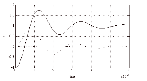
We could also plot all three components of x by using plot(t,x), as shown in Fig. 2.

Fig. 2. Graph of the state vector x versus time for the circuit of Fig. 1.

If tf is chosen to be too large, the matrix size limitation in the student edition of Matlab^® will be exceeded. Also, sometimes choosing tf to be too large will cause a message "singularity expected," and the function will not be executed.

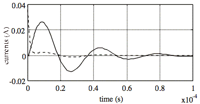
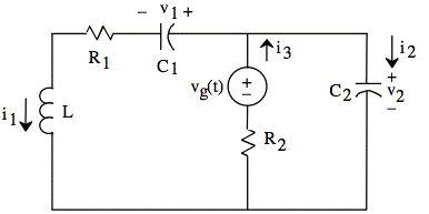
Ex:           Use ode45 to solve for x for the circuit in Fig. 3 when R1 = 20 Ω, R2 = 5 Ω, C1 = 100 nF, C2 = 200 nF, L = 300 μH, vo = 1 V. Then plot i1 versus t and i3 versus t.

     

   Fig. 3. The voltage vg(t) changes instantly from −vo to vo at t = 0.

Given:                     x = [i1 v1 v2]'

                dx1/dt = (x3 − x2)/L − x1 R1/L

                dx2/dt = x1/C1

                dx3/dt = −x1/C2 + (vg − x3)/(R2 C2)

                                  xo = [0 −vo −vo]'

Ans: